SEO specialists work with large data sets almost every day. In a typical SEO report, hundreds and thousands of data strings must be created, updated, organized, exported, and analyzed. How can you ensure speed and accuracy at the same time? Doing it manually is not the best option. So, you should know Excel & Google Sheet Tips For SEO.
The reason is Google Spreadsheet functionality comes to the rescue. It provides convenience and speed, supporting our daily SEO tasks. The best part, however, is Google Sheets’ (or Excel) ability to automate data maintenance, processing, and calculations.
Today, I will give you several useful Excel & Google Sheets functionality tips to ease your SEO routine.
Best Excel & Google Sheet Tips For SEO Data
In the under section, I have mentioned some highly functional Excel & Google Sheet Tips For SEO for better results.
Tip #1. Use Keyboard Shortcuts to Streamline Work With Data
Keyboard shortcuts are named that way for a reason: they provide the shortest routes to solving problems or achieving the desired outcome. Shortcuts are useful when performing repetitive actions, like selecting ranges, filtering, or sorting data.
Some of the most widely used keyboard shortcuts for working with Google Sheets for SEO:
- Ctrl+Shift+E (Open Explore Panel)
- Ctrl+Shift+7 (Add Border)
- Ctrl+Alt+Shift+H (Insert Note)
- Ctrl+Alt+Shift+M (Insert Comment)
- Ctrl+Alt+Shift+R (Refresh Data)
- Ctrl+\ (Remove Formatting)
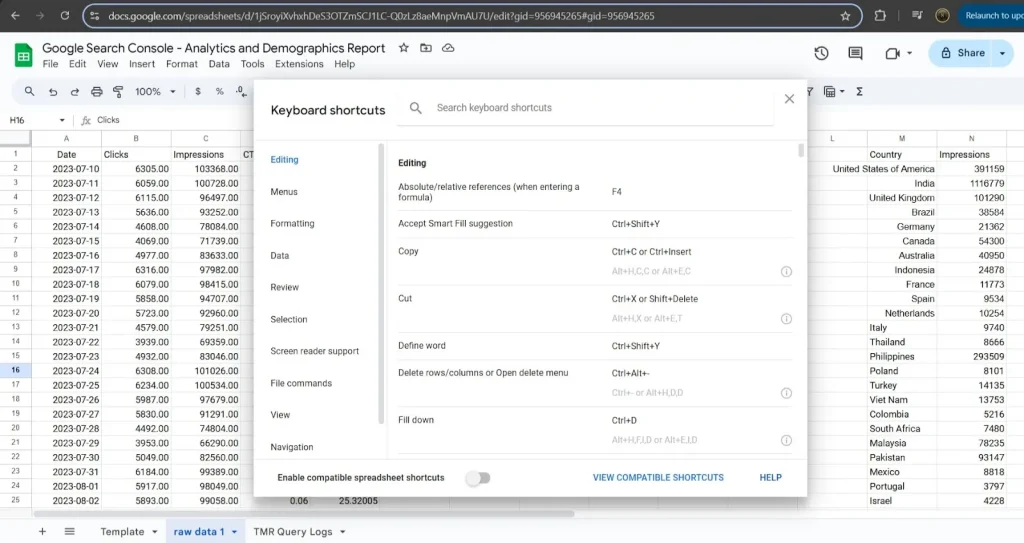
If you want to see all the available shortcuts, use this combination of buttons: Ctrl+/. A window will pop up with a detailed overview and description of all shortcuts, plus you can use a handy search function at the top.

Tip #2. Use Duplicate Identification Function for Spam-Free Link Building
Link building is a time-tested and reliable strategy for outreach in SEO and digital marketing. Despite the recent shifts to the quality of content and user intent fitness, link building remains the main pillar of success in on-page and off-page SEO.
However, it’s not as simple as it seems — whether you know how to get quality backlinks for free or buy backlinks, you still need to filter out vast amounts of domain data, ensuring no duplicates remain and all the entries are unique.
This is where our Excel & Google Sheet Tips For SEO become handy; namely, the Google Sheet function =COUNTIF(range, criteria) enters the stage.
It allows you to quickly identify domain duplicates or email address duplicates in your outreach template. Before reaching out to webmasters, you can be sure that you won’t contact someone twice or even three or more times.
For instance, if your outreach contact data is in column A and you want to check for duplicates of cell A1, the formula will be:
=COUNTIF(A:A, A1)
You only need to take three easy steps to identify duplicates in a SEO report:
- Enter the above-mentioned formula in the adjacent to your data column.
- Drag the formula down to evaluate all rows (left mouse button pressed).
- Filter or highlight rows with values greater than 1 (indicating duplicates).
The utility of this function for you as an SEO specialist is that it saves your time and prevents reputation damage caused by spammy outreach.
Tip #3. Apply Conditional Formatting for Better Analysis and Insights
When you see a vast database with thousands of entries, it’s easy to get lost and overlook the important things. To aid SEO and marketing experts in analyzing data, Google Sheets and Excel have a helpful functionality — conditional formatting.
Its main function is formatting or highlighting a data set or separate cells based on a pre-defined (and custom-made) rule.
This is how to activate conditional formatting:
- Select the Range: Highlight the cells or range by left-clicking and dragging the mouse.
- Open Conditional Formatting:
- Go to Format in the main top menu.
- Select Conditional Formatting.
- Set a Rule:
- A window will open on your right-hand side. In the Format Rules section, select a predefined rule or use a custom formula.
- Customize: Choose your preferred formatting style (font type and size, text color, background color, etc.).
- Apply: Click Done to save the rule.
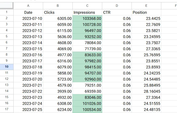
On this screenshot, we’ve applied conditional formatting to impressions. The intent was to highlight impression values greater than 8000 with a green color.

Other examples of conditional formatting applications in SEO:
- Backlink Quality Analysis. For example, you can highlight only the domains with DA/DR values above 50.
- Keyword Performance Tracking. For example, highlight click-through rates (CTR) below 10% with red color.
- Technical SEO Checks. For example, make page loading times with values that are too high easily visible.
In utilizing Excel for SEO purposes, you can also use conditional formatting for better social mentions sentiment analysis. However, first, you must know how and where to get all the data. For that, you may want to look at this page, which shows multiple methods marketers can use to collect data for sentiment analysis.
Tip #4. Conveniently Track Rankings Over Time
Google Sheets has a powerful functionality for retrieving specific data from a larger volume of data. In SEO and digital marketing in general, it can be very helpful when the goal is to track specific values (such as rankings) over time.
Formula basics:
=VLOOKUP(lookup_value, table_array, col_index_num, [range_lookup])
- lookup_value: specifies the keyword you want to track.
- table_array: defines the range of your data/values containing keywords and rankings.
- col_index_num: sets the column number where the required data is located.
- range_lookup: e.g., you can apply FALSE for an exact match.
A step-by-step example:
- Set Up Your Data:
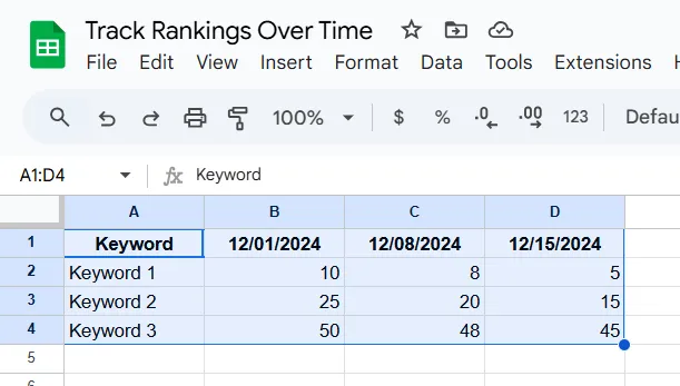
Make a table with keywords (A column) and relevant rankings across different dates, like so:

- Retrieve Rankings:
Use VLOOKUP command to find a specific keyword’s ranking:
- Formula:
=VLOOKUP(“Keyword 1”, A1:D4, 3, FALSE) - Explanation:
- “Keyword 1” is the keyword you want to locate.
- A1:D4 is the data range you want to include (basically, the whole table).
- Value 3 indicates that the result should come from the third column, “C” (12/08/2024).
- FALSE finds an exact match for the relevant keyword.
- Result:
Our function returns the ranking for “Keyword 1” on 12/08/2024, which is 8.
Possible SEO spreadsheet application scenarios for the VLOOKUP
- Monitor Individual Keyword Performance. It enables you to focus on the most critical keywords for your SEO project/campaign goals.
- Identify High-Performing Keywords. Save time and money by focusing efforts only on high-performing keywords.
- Troubleshoot Ranking Drops. Quickly see which data parameters in your SEO activity require more attention.
Here is a summary of the benefits that the VLOOKUP function can provide. Firstly, it can boost efficiency by empowering you to instantly locate the high-performing or underperforming rankings. Secondly, it ensures a precise retrieval of keyword data from a large dataset. And lastly, it makes your work easier by amplifying your ability to work with large datasets.
The Bottom Line
Current Excel and Google Sheets tips and basic functions will be useful for SEO specialists and digital marketers alike. They enhance speed, improve data utility, and facilitate collaboration when a group of colleagues has to work on a single database.
However, we cannot cover all the functions and tricks of Google Sheets for SEO purposes in this article, as there are just too many of them. Therefore, we encourage you to explore this topic further by starting with topics adjacent to the ones covered today.


